Weiss B, Clemens Zs, Bódizs R, Halász P: Comparison of fractal and power spectral EEG features: Effects of topography and sleep stages. Brain Res Bull 84(6):359-75 (2011)

DOI:10.1016/j.brainresbull.2010.12.005

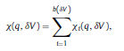
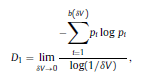
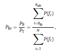
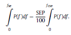
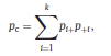
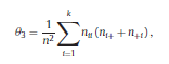
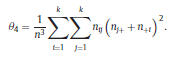
Béla Weiss^a, Zsófia Clemens^b, Róbert Bódizs^c,d, Péter Halász^a

^aFaculty of Information Technology, Pázmány Péter Catholic University, Práter u. 50/a, 1083 Budapest, Hungary
^b National Institute of Neuroscience, Amerikai út 57, 1145 Budapest, Hungary
^c Institute of Behavioural Sciences, Semmelweis University, Nagyvárad tér 4, 1089 Budapest, Hungary
^dHAS–BME Cognitive Science Research Group, Stoczek u. 2, ST. Building, III/311, 1111 Budapest, Hungary

ABSTRACT

Fractal nature of the human sleep EEG was revealed recently. In the literature there are some attempts to relate fractal features to spectral properties. However, a comprehensive assessment of the relationship between fractal and power spectral measures is still missing. Therefore, in the present study we investigated the relationship of monofractal and multifractal EEG measures (H and D) with relative band powers and spectral edge frequency across different sleep stages and topographic locations. In addition wetested sleep stage classification capability of these measures according to different channels.We found that cross-correlations between fractal and spectral measures as well as between H and D exhibit specific topographic and sleep stage-related characteristics. Best sleep stage classifications were achieved by estimating measureD in temporal EEG channels both at group and individual levels, suggesting that assessing multifractality might be an adequate approach for compact modeling of brain activities.

Keywords

Fractal analysis; Power spectral analysis; Topography; Cross-correlation; Sleep stage classification

1. Introduction

With advent of relatively cheap and high performance personal computers sophisticated and computation demanding time series analysis methods became available to a broad brain research community. Application of chaos theory and non-linear time series methods gave a deeper insight into brain dynamics reflected by EEG signals. For a comprehensive recent review on non-linear analysis of EEG we refer to ref. [90]. This approach relies on a transition from the time domain to the phase space and generation of trajectories for EEG time series using different embedding techniques. Inferences about brain dynamics were drawn by estimating different characteristics of trajectory attractors using measures such as the correlation dimension D2, the fractal dimension Df, the largest Lyapunov exponent L1, etc. Early results were promising and suggested a deterministic nature of brain dynamics with a rather low-dimensional chaotic behavior in physiological and pathological conditions that could not be revealed using simple linear methods such as power spectral analyses. Filtered noise, however,can mimic the signatures of deterministic chaos [77]. This latter finding necessitated a revision of results obtained by non-linear techniques. Surrogate data analyses [83] did not entirely support early results on the low-dimensional chaotic behavior of the brain. This was in agreement with the finding that the relatively high complexity of the EEG signals does not allow a reliable dissociation of its waxing and waning oscillations exceeding 2–15 s from that of the filtered white noise [14,69,89]. As a consequence alternative approaches were developed including novel non-linear and stochastic time series analysis methods.
Fractality is a common property in nature [65] which may originate from self-organized criticality (SOC) [4–6] of the particular system of interest. Unlike deterministic approaches aimed at finding low-dimensional chaos, the SOC framework allows for describing the high-dimensional character of the dynamics and the presence of stochastic effects [58]. SOC is a phenomenon characterizing systems that might arrive at a critical state (phase transition) without any tuning of a specific parameter [6]. The proof of presence of SOC requires a demonstration of spatio-temporal long-range correlations and power-law scale-free (also called selfsimilar or fractal) fluctuations [4]. Scale-free behavior means that no characteristic scales dominate the dynamics of the underlying processes. It also reflects a tendency of complex systems to develop correlations that decay more slowly and extend over larger distances in time and space than the mechanisms of the underlying processes would suggest [4,7,8,58]. The long-range correlations build up through local interactions until they extend throughout the entire system. After this stage, the dynamics of the system exhibit power-law scaling behavior and the underlying process operates in a critical state [5,6]. A critical state is a regime of a system where opposing forces are balanced. In the nervous system such a balance might be represented by the relationship between excitation and inhibition, which is known to be important for the transfer of information [85] and for the sustained neuronal activity [87]. Neural network simulations demonstrated that the presence of long-range spatio-temporal correlations is beneficial for the optimal transfer of information since these correlations represent an optimal compromise between high susceptibility to perturbations and stability in the system [10,17].
Several features of neural networks are consistent with SOC, such as a large number of elements (neurons) interacting with each other in a nonlinear way (e.g. presence of threshold for spiking), a possibility to change and save connectivity between the elements (e.g. via synaptic plasticity), absence of any special parameter tuning, and spatio-temporal dynamics obeying power-law statistics [58,68]. Despite of these common properties of neural networks and SOC systems, several studies revealed power-law neural fluctuations that do not necessarily reflect self-organized critical states of brain [9,80,81]. For example, Bédard et al. [9] have shown that fractal property of local field potentials recorded from cat parietal cortex does not rely on critical states, but rather stems from filtering properties of the extracellular media. All these results indicate a more general nature of fractality that could be used as a descriptor of structural and functional properties of the brain during different conditions.
Fractal geometry of brain structures [49,70] as well as powerlaw spatio-temporal properties of neuronal activities have been revealed. Although the spatial power spectral density (PSDx) of scalp EEG recordings might deviate from the ideal power-law scalefree behavior [34], the PSDx of epipial EEG conforms to it [33]. Temporal long-range correlations were observed at different levels of the brain electrical activity hierarchy in different species and during different conditions. For example, Lowen et al. revealed that individual ion channel currents show long-term correlation and possess fractal properties [62]. Considering spike trains in extracellular recordings, long-term correlations were found among interspike intervals of the medullary sympathetic neurons in cats [56]. Spasic et al. showed that the fractal dimension of local field potentials of anaesthetized rats changes significantly after unilateral discrete injury [88]. Fractal exponent of EEG activity in the Gallotia galloti lizard decreased with the increment of temperature from 25 ◦C to 35◦C [35].
The exact values of fractal measures may be related to biophysical mechanisms and the neural architecture underlying oscillations. However, given the uncertainties related to the estimation of these measures [15,16,36,42,47,48] it might be more reasonable to compare the variances of features for different conditions. In line with this, a series of human studies revealed differences in the fractal measures between specific conditions. A study by Linkenkaer- Hansen et al. [58] showed that mu and alpha oscillations scale similarly, but beta oscillations have a significantly smaller scaling exponent compared to these two latter oscillations during eyes-closed state. Another study showed that long-range temporal correlations are stronger in the eyes-closed condition as compared with the eyes-open condition [67]. In the study of Nikulin and Brismar [68] largest exponent values for alpha and beta oscillations were found during the eyes-closed condition in the occipital and parietal areas. Fractal dimension was found to be significantly higher for drowsy EEG compared to the wake state [13]. Increased sensory input [59] or high level of alertness [75] was shown to disrupt long-range temporal correlations. Several studies addressed self-similarity of sleep EEG [1,53–55,63,74,86,95]. Generally, most of these studies reported higher scaling exponents and thus stronger long-range temporal correlations for deeper sleep stages. It was also indicated that brain electrical activities are more complex than they could be completely described by a single scaling exponent [63,95]. In a previous study [95] we provided a detailed topographic analysis of temporal fractal measures during different vigilance states. In the present study we extended the characterization of self-similarity properties by a comprehensive topographic comparison of multifractal and monofractal measures with each other and with power spectral measures, and also examined their sleep stage classification capabilities.

2. Materials and methods

2.1. Subjects and EEG recordings

Twenty-two healthy subjects with no sleep disturbances, free of drugs and medications as assessed by an interview and questionnaires on sleeping habits and health participated in the study (age: 17–55 years, mean±S.D.: 31±9 years, 11 males and 11 females). The study was approved by the ethical committee of the Semmelweis University and subjects gave written informed consent to participation. Sleep was recorded in the sleep laboratory for two consecutive nights. The timing of lights off was determined by the subjects, and morning awakenings were spontaneous. On average subjects spent 462.39±69.01 (mean±S.D.) minutes in sleep during the second night. Sleep was recorded by standard polysomnography, including electroencephalography (Fp1, Fp2, F3, F4, Fz, F7, F8, C3, C4, Cz, P3, P4, T3, T4, T5, T6, O1 and O2 electrodes), electrooculography (EOG), bipolar submental electromyography (EMG) and electrocardiography (ECG). EEG electrodes were referenced to the contralateral mastoid. Midline EEG electrodes were referenced to the right mastoid. Impedance of the EEG electrodes was kept below 5 k. Signals were collected, pre-filtered, amplified and digitized at a sampling rate of fs = 249 Hz using the 30 channel Flat Style SLEEP La Mont Headbox with implemented second order filters at 0.5 Hz (high pass) and 70 Hz (low pass) as well as the HBX32-SLP 32 channel preamplifier (La Mont Medical Inc., USA). Additionally, a 50Hz digital notch filtering was performed by means of the DataLab acquisition software (Medcare, Iceland).

2.2. EEG processing

Pre-processing and feature estimation were accomplished in a self-developed EEG visualization and processing toolbox under Matlab2009b (MathWorks, Natick, MA,USA). Statistical analyses were performed using STATISTICA (StatSoft, Inc., Tulsa, OK, USA) and Matlab2009b.

2.2.1. Pre-processing
Although hardware filtering had been applied during EEG recording, some artifacts remained. Thus, we first performed software filtering on the raw EEG recordings with Butterworth IIR filters (eight order 0.3–70 Hz band-pass and 50 Hz notch with a quality factor Q= 45). To avoid phase distortion, we used the built-in filtfilt( ) function of the Matlab for zero-phase digital filtering. For all subjects a hypnogram was prepared according to the Rechtschaffen and Kales standard [78] using 20 s long epochs. To compare the analyzed EEG features during different sleep stages 90 epochs of 20 s length were selected from sleep stages NREM2, NREM4 and REM (30 min/stage) for all subjects. Selection included segments without artifact contamination only.

2.2.2. Fractal analysis
Monofractal and multifractal properties of the selected EEG epochs were evaluated by estimation of the self-similarity parameter H (also called Hurst exponent or Hurst parameter) and the range of fractal spectra (D), respectively. To estimate H, we applied the rescaled adjusted range based approach, while D was approximated by estimation of generalized dimensions spectra. The brief description of the applied methods can be found in the following subsections. For detailed information on selection of estimation methods and parameter settings we refer to [95].

2.2.2.1. Estimation of the Hurst exponent.
The stochastic process X(t) with continuous parameter t is self-similar with the self-similarity parameterHif the distribution of the rescaled process c^−HX(ct) is the same as the distribution of X(t), where c>0 is arbitrary [64]. H is widely used to assess monofractality, scale-free properties and the degree of long-range temporal correlations of time series.When 0 < H < 0.5, an increase in the process is more probably followed by a decrease (anti-persistence) and vice versa, the process is considered to have short-range dependence. If H= 0.5, observations of the process are uncorrelated. When 0.5 < H < 1, an increase in the process is more probably followed by an increase and a decrease is more probably followed by a decrease (persistence), the process is considered to have long-range dependence [1,12,44,47,64].
Basically two kinds of homogenous self-similar (see also the first paragraph of Section 2.2.2.2) signals exist: fractional Gaussian noises (fGn) and fractional Brownian motions (fBm). fGn processes are considered to be stationary with a constant mean value and constant variance over time, while fBm’s exhibit non-stationary property with a time-dependent variance. fGn and fBm signals are interconvertible. Taking the differences between neighboring elements of an fBm time series one might create an fGn signal, while by cumulative summation of fGn elements one can generate a motion process. The corresponding fBm and fGn signals are characterized by the same H. Self-similarity of a time series is also reflected in their power spectrum. The power versus frequency relationship is given by P(f)∝f^−K, where K is called spectral or fractal exponent. Depending on the type of a fractal signal the relationship between H and K is given by H= (K + 1)/2, −1< K < 1 for fGn and H= (K −1)/2, 1< < 3 forfBm[26]. Similarly,H is linearly related to the detrended fluctuation analysis exponent [71,72] as H= λ for fGn signals and H= λ−1 in case of fBm processes. Additionally, the Hurst exponent is also related to the widely used fractal dimension as H=2−Df [25,41], where Df refers to the fractal dimension of a one dimensional Brownian motion X(t) in the X–t plane. Although many approaches are available for the estimation ofHnone of these can be generally considered as an ideal one because of differences of fGn and fBm signals [24–26,76] and doubts related to the estimation of non-linear parameters from time series of finite length [15,16,36,42,47,48]. Like in our previous study [95] for the estimation of H we used the rescaled adjusted range or R/S statistics based method [12,44,64].We implemented this method keeping in mind the stationarity properties of the analyzed EEG segments and the fact that this method is applicable to stationary fGn processes or to differenced fBm signals only. Here we provide a short description of this approach, for further details we refer to [95]. Let X(n) be a discrete time series. The partial sum process is defined as

The sample variance of the process X can be obtained using

The adjusted range is given by

where


The R/S statistics or the rescaled adjusted range is defined by

In [64] it was proven that for self-similar processes the expected value of R/S(n) is proportional to n^H, i.e.

as n→∞, where CH is a positive constant and H is the self-similarity parameter of the process. Using this power-law relationship the Hurst exponent can be estimated by:

2.2.2.2. Estimation of multifractal spectra.
Homogenous self-similar time series can be described by a single scale-free exponent. These signals are also called monofractal time series. Additionally, heterogeneous multifractal time series showing self-similarity only in local ranges of the structure also exist. Their scale-free property varies in time. Hence they should be decomposed into many sub-sets and characterized by different exponents. This can be carried out by estimation of fractal spectra. Using the Alfréd Rényi’s generalized entropy, a continuous spectrum of generalized dimensions (also called Rényi dimensions or fractal spectrum) D_q can be defined, where −∞≤q≤∞[79]. A commonmethod for estimation of fractal spectra is the box-counting technique. In this study we applied a box-counting approach that is based on estimation of the moments of signal amplitude distribution and was also used in [51,95]. One reason for choosing this method is that a previous study [28] revealed a promising sleep stage classification performance of entropy of amplitudes (ENA), a measure that is closely related to the amplitude distribution of time series. In our case D_q is defined as follows:

δV is the bin width or box length. The partition function can be obtained using

where b(δV) denotes the number of non-overlapping bins

V_max and V_min are themaximumand minimum values of EEG signals recorded during measurements, respectively. Χ_i(q, δV) = p^q_i is a weighted measure that represents the percentage of EEG values that falls into the ith bin, and q is the moment or weight of the measure. If n_i is the number of EEG values in the ith bin and N is the total number of the samples, than the probability that the signal falls into the ith bin of length δV is:

Some of the D_q values are known under different names and widely used in the field of time series analysis. D₀ is the Hausdorff-Besicovitch or fractal dimension. For q = 1 one should use

where the numerator is the well-known Shannon’s entropy and can be related to ENA applied in [28]. D2 is called correlation dimension.
The range of fractal spectra is defined as ΔD= max(D_q)−min(D_q), where max(D_q) =D_−∞, min(D_q) =D_∞, i.e., ΔD=D_−∞ −D_∞, since D_q is a monotonically decreasing function. ΔD is a measure of multifractality, indicates deviation from monofractal. Larger ΔD indicates multifractality, while smaller ΔD indicates that the analyzed system tends to possess the monofractal property.

2.2.3. Power spectral measures (PSMs)
To assess the relationship between fractal measures and power spectral properties of sleep EEG signals, we estimated the relative power of widely used frequency bands (RBPs). Relative powers were used instead of absolute ones in order to avoid the effect of variation of total power across subjects. To describe spectral properties in a more compact way, we calculated the spectral edge frequency (f_se) since this measure can be considered as a clinically well-established EEG measure for monitoring sleep cycles and depth of anesthesia [28,37,38,61].
Before estimation of power spectral EEG features, Hanning windowing was applied to the selected epochs to damp out the frequency leakage, i.e., the Gibbs phenomenon that originates from truncation of time series. From these windowed time series the power spectra P(f) were obtained using the Fast Fourier Transformation (FFT) with frequency resolution f = 0.152 Hz and range [0Hz, f_s/2Hz]. The relative power of the B frequency band can be calculated from a power spectrum as follows:

where P_T is the total power of the time series, P_B is the total power of the B frequency band, f_i = (i−1)Δf with a maximal value of f_s/2 when i =N, B_ub and B_lb are indices corresponding to the upper and lower boundary frequencies of the B band, respectively. The analyzed bands were as follows: SO: (0.5–1] Hz, δ: (1–4] Hz, Θ: (4–8] Hz,α: (8–11] Hz, σ : (11–16] Hz, β: (16–30] Hz, γ: (30–70] Hz. These frequency bands are thought to represent specific EEG patterns. Slow oscillations (SOs) were assessed separately from delta band activity given their distinct characteristics [3,66].
The spectral edge frequency was defined as the frequency up to which SEP% of the total power of the [0Hz, f_cse Hz] frequency range is accumulated:

In this study SEP and cut-off f_cse frequency parameters were set to 95% and 70 Hz, respectively. According to Eq. (14) and the nature of sleep EEG, lower f_se values can be predicted for deeper sleep stages since during these states the power spectrum is biased towards lower frequencies.

2.3. Statistical analysis

2.3.1. Topographic distribution of EEG measures across different sleep stages
Normality of the estimated features was tested using the Shapiro-Wilk W test, while the homogeneity of variances was evaluated with the Levene test. Since not all of the estimated measures matched normality and homogeneity in each channel we evaluated the effect of sleep stages using the non-parametric one-way Kruskal–Wallis analysis of variances (ANOVA). Individual medians of the estimated measures were grouped using the independent variable “STAGE” having factors levels NREM4, NREM2 and REM. Pair-wise comparison of sleep stages was carried out with rank post-hoc test. To test differences between bilateral symmetric scalp locations we used the Wilcoxon matched pairs test for each measure and sleep stage. For this purpose eight symmetrical channel pairs (Fp1–Fp2, F7–F8, F3–F4, C3–C4, T3–T4, T5–T6, P3–P4, O1–O2) and an additional midline channel pair (Fz–Cz) were formed.

2.3.2. Cross-correlation analysis
Cross-correlations were calculated between locations for all estimated measures (inter-site correlations) and between the measures at each location. Specifically, comparisons were carried out between monofractal and multifractal measures as well as between fractal and power spectral features. Spearman’s correlation coefficients were calculated in all cases using individual medians of particular EEG measures. Sleep stages were considered separately as well as together.

2.3.3. Hierarchical clustering
Effect of topography was analyzed by hierarchical clustering of channels for all three sleep stages. Z-score standardization of the individual medians was carried out for all measures and channels separately. Hierarchical channel cluster trees were generated by pairing eight similarity measures (Euclidean distance (euc); standardized Euclidean distance (seu); Mahalanobis distance (mah); city block metric (cit); Minkowski metric (min); cosine distance (cos); correlation distance (cor); Chebychev distance (che)) with seven linkage methods (unweighted average distance (ave); centroid distance (cen); furthest distance (com); weighted center of mass distance (med); shortest distance (sin); inner squared distance (war); weighted average distance (wei)). Performance of each combination was assessed by calculation of the cophenet correlation coefficient (CCC). We selected the similarity-linkage pair with highest CCC value to cluster the channels into four and nine clusters. The 4-cluster analysis was aimed to reveal possible groupings of neighbor EEG channels and thus forming e.g. anterior, posterior, central, lateral or similar clusters. The 9-cluster analysis was applied to assess whether symmetrical EEG channels (see Section 2.3.1) also cluster together.
Clustergrams were generated for measure and channel clustering using group level medians (medians of individual medians) of all measures in all channels. Standardization of features was performed across channels. Clustergrams, enclosing heat maps and dendrograms were examined for sleep stages separately. Hierarchical channel cluster trees were generated using the cosine similarity metric and the unweighted average linkage method. Measure dendrograms were constructed applying the Euclidean distance as a similarity measure and the unweighted average method for linkage. Channel clustering was also carried out based on the two fractal measures as well as combining the seven relative band powers.

2.3.4. Linear discriminant analysis
Classification of sleep stages was performed with linear discriminant analysis (LDA) using all features and all channels separately both at individual and group levels. At the individual level 3×90 estimated values were used for each subject, while 22×3×90 values were considered at the group level. After a 10-fold cross-validation procedure the accuracy of classifications was assessed with Kappa analysis of the confusion (also called error) matrices.

2.3.4.1. Confusion matrix.
A confusion matrix C is a k×k quadratic matrix, where k is the number of classes. Columns of C stand for the reference data (classification performed by the human expert in this case) and rows denote the classified data (LDA classification in this case). Hence, Cij = nij is a count of EEG segments classified by the human expert into the jth class but classified to the ith class using LDA. For an example see Table 1 that presents the confusion matrix obtained by LDA classification of sleep stages usingD measure in the Cz channel of a representative subject #16. The number of segments classified to the ith class using LDA is

while

is the total number of segments classified to the jth sleep stage by the human expert. Let p_i,j denote the proportion of samples in the i, jth cell of C, corresponding to n_i,j:

where n is the total number of the analyzed EEG segments. Furthermore, marginals p_i+ and p_+j can be defined by

and

2.3.4.2. Kappa analysis.
The Kappa analysis is a technique used to statistically test whether two confusion matrices are significantly different. The result of Kappa analysis is a KHAT statistic ˆK, an estimate of Kappa that is a measure of classification accuracy or agreement. It is based on the difference of the actual agreement (the major diagonal of the error matrix) and the chance agreement (indicated by the row and column totals, i.e. marginals). If the actual agreement is

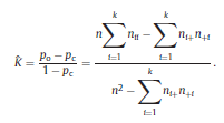
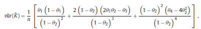
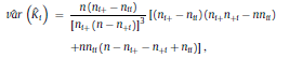
and the chance agreement is defined as

the estimate of Kappa is given by

The variance of Kappa is as follows:

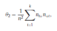
where

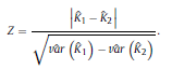
and

ˆK can take values from the range [−1, 1]. However, positive values are expected since there should be a positive correlation between classifications performed by the human expert and LDA. Landis and Koch characterized the possible ranges for KHAT into three groups [52]: a value greater than 0.80 (i.e., >80%) represents strong agreement; a value between 0.40 and 0.80 (i.e., 40–80%) represents moderate agreement and a value below 0.40 (i.e., <40%) represents poor agreement. As it can be seen in Table 1, a strong agreement (ˆK = 0.85) between classifications performed by the human expert and LDA was found using the ΔD measure in the central channel of subject #16.
It was shown that the Kappa analysis overestimates the proportion of randomness and thus underestimates the classification accuracy [18,19]. Therefore, where applicable, we also provide the most widely used classification performance measure, the overall accuracy

For the particular confusion matrix presented in Table 1 with ˆK = 0.85, the corresponding overall accuracy was 90.37%.

The fact that the ˆK statistic is asymptotically normally distributed provides a means for testing the significance of ˆK for a single confusion matrix to determine if the agreement between the classification performed between the human expert and LDA is significantly grater than zero, i.e., LDA performs better that than a random classifier. The test statistic is expressed by:

Given the null hypothesis H₀ : K = 0, and the alternative H₁ : K ≠ 0, H0 is rejected if Z ≥ Z_α/2, where α/2 is the confidence level of the two-tailed Z test.

Moreover, there is a test to determine whether two confusion matrices are significantly different. This provide us the opportunity to compare classifications performed using different EEG features and channels. Let ˆK₁ and ˆK₂ ( var(ˆK₁) and var(ˆK₂) ) denote the estimates of the ˆK statistic (estimates of variances) for confusion matrices #1 and #2, respectively. The test statistic in this case is defined as

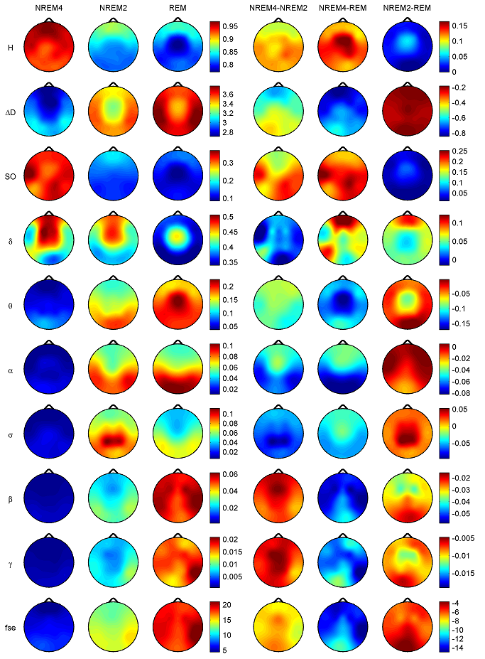
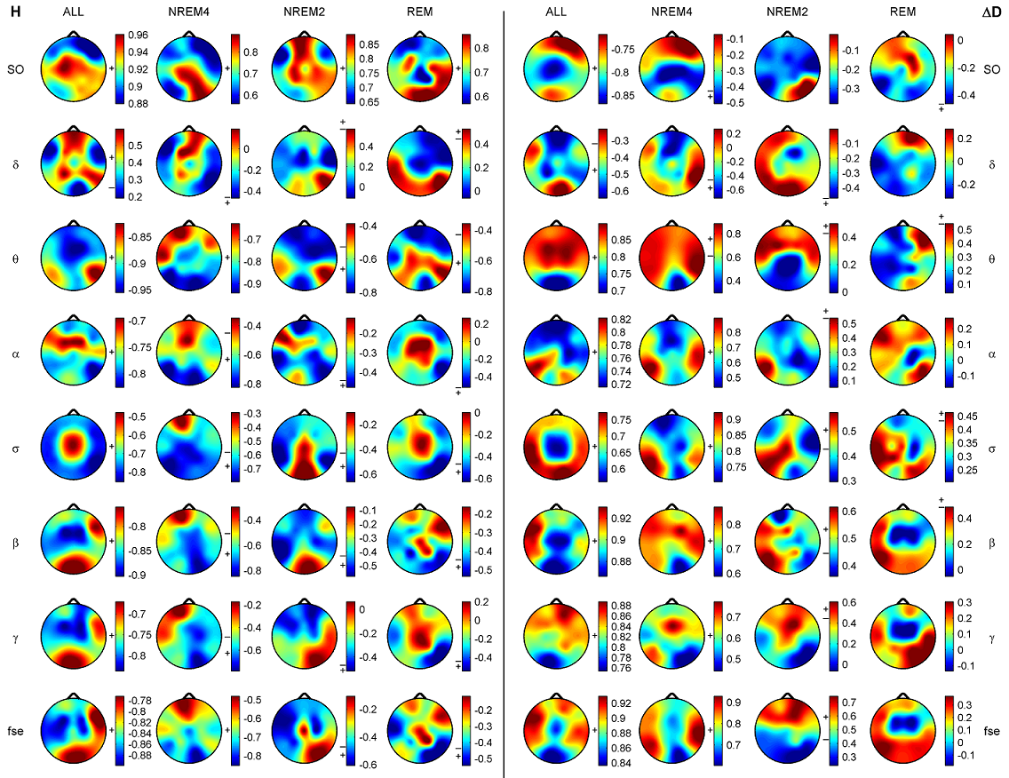
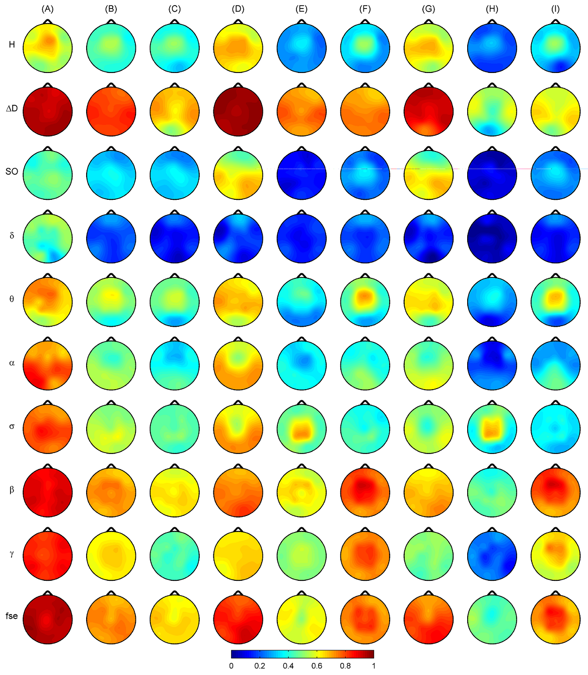
Z is standardized and normally distributed. Given the null hypothesisH₀ : K1 −K2 =0, and the alternative H₁ : K1 −K2 ≠ 0, H0 is rejected if Z ≥ Zα/2.
Finally, in addition to computing statistics for an entire confusion matrix, it may be useful to look at the agreement of individual classes. Individual class accuracy can be tested using the conditional Kappa coefficient. The estimates of the conditional Kappa coefficient and its variance for the ith class are given by

and

respectively. The same comparison tests available for the Kappa coefficient apply to this conditional Kappa for an individual class. For more details and comparison of Kappa analysis to other methods we refer to [18,19].

3. Results

3.1. Distribution of EEG measures across vigilance states and topographic locations

Topographic distributions of group level medians for the three sleep stages as well as their differences are shown in Fig. 1. Results obtained for the fractal measures were in agreement with those presented in [95]. Namely, highest H values emerged frontally during all sleep stages, while the minimum was found during REM in the central zone. A H_NREM4 >H_NREM2 >H_REM trend was present across the whole head surface. Measure ΔD, showed an opposite trend: D_REM >D_NREM2 >D_NREM4. Minima of ΔD could be found in the fronto-central region during all sleep stages, while higher values were observed in the posterior circumferential channels. Salient H difference peaks that occurred for sleep stage pairs NREM4-REM and NREM2-REM could not be observed in the case of ΔD. Power spectral measures also exhibited expected topography. Relative band powers of slow activities (SO and δ bands) were higher for NREM4 than NREM2 as well as for NREM2 than REM. Generally, P_SOr showed amore even topographic distribution when compared to P_δr in all sleep stages. Across all sleep stages the minimum of P_SOr occurred at the vertex during REM sleep. Frontal regions exhibited slightly higher values of P_SOr compared to other regions during NREM2 and REM. During NREM4 higher P_SOr values occurred bilaterally in the fronto-temporal region and in C4, P4, O2 channels. P_δr exhibited higher values in the fronto-central channels during NREM4 and NREM2 and in the central region during REM sleep. Generally, faster activities (above 4 Hz) showed an opposite trend with lower relative band power values for deeper sleep stages. During NREM4 relatively even topographic distributions were found for faster activities. During NREM2 higher values appeared in the posterior region, showing maxima in the parietal channels for P_δr. REM sleep revealed a more diverse topography of faster activities. Maximum of theta activity was found centrally. Highest values in the α and σ bands occurred in posterior channels. Finally, relative power of β and γ frequency bands peaked in temporal channels. Spectral edge frequency showed lower values for deeper sleep stages as it was conjectured from Eq. (14). Slightly higher values of f_se were present in posterior channels during NREM4 and NREM2, while during REM higher values were located in temporal channels.

Comparing sleep stages using one-way Kruskal-Wallis ANOVA revealed highly significant (p < 0.00001) differences for all measures in all channels except for the relative power of the δ band. For detailed results see the supplementary Table S1. The level of significance for P_δr varied across channels between p < 0.01 and p < 0.00001. Pair-wise comparison of sleep stages using the rank  post-hoc test resulted in most significant differences between sleep stages NREM4 and REM for all measures and channels with the exception of P_σr. This latter measure exhibited highest significance values between NREM4 and NREM2 in fronto-centroparietal channels (F3, Fz, F4, C3, Cz, C4, P3 and P4). In general, least or non-significant differences were observed between sleep stages NREM2 and REM. Comparison between NREM4 and NREM2 revealed significant values for all measures with the exception of the relative δ band power which reached significancy in F3, C3, P3 and P4 channels only.

Fig. 1. Topographic distribution of group level medians (medians of individual medians) for the analyzed sleep stages and differences of these medians between sleep stages. Relative band powers are denoted by the labels of the corresponding frequency bands.

3.1.1. Interhemispheric comparisons

As expected, Wilcoxon matched pairs test revealed (Table 2) more significant differences for the non-symmetric Fz–Cz channel pair as compared with the other symmetric channel pairs. Out of the 30 cases (10 measures×3 stages) the Fz–Cz channel pair exhibited 19 significant values. Regarding the symmetric channel pairs most significant differences were found for channel pairs P3–P4 (10 cases) and O1–O2 (8 cases), while least significant differences appeared for the frontal channel pairs Fp1–Fp2 (2 cases), F7–F8 (4 cases) and F3–F4 (4 cases). In posterior channel pairs more significant results occurred during deeper sleep stages while in frontal channel pairs the least significant differences were found during sleep stage NREM4. Most significant interhemispheric differences occurred for relative powers of delta and beta frequency bands (7 cases for both out of total 24 = 3 sleep stages×8 symmetrical channel pairs). For P_δr significant cases were distributed similarly across sleep stages, while P_βr revealed the most (5 cases) significant differences for NREM2 sleep. P_SOr resulted in 4 significant cases, all during NREM4. By contrast, no significant interhemispheric differences were found for P_γr in this sleep stage. No gross tendencies were observed for P_αr and P_σr across sleep stages and locations, however, there were some significant results. Compact EEG features (H,ΔD and f_se) altogether revealed a lownumberof significant results: 5, 4 and 0 significant cases for NREM4, NREM2 and REM, respectively.
Considering all 10 measures NREM2 (20 cases) and NREM4 (17 cases) revealed twice more significant differences as compared to REM sleep (8 cases out of total 80 = 10 measures×8 symmetrical channel pairs).

3.2. Cross-correlation analysis

3.2.1. Inter-site correlations
In Fig. 2 the 35 strongest inter-site correlations (p < 0.05) are denoted by black lines drawn between the appropriate locations for all 10 EEG measures and for each sleep stage separately as well as together (also see Supplementary video Inter_site_correlations.avi for different number of inter-site correlations). Considering all sleep stages together highest inter-site correlations were observed centrally (F3, Fz, F4, C3, Cz, C4, P3, P4) for all features except for the relative power of the band where highest correlations were found intrahemispherically. Sleep stages were characterized by different topography in inter-site correlation maps. In general, power spectral measures (except for P_γr) showed strongest correlations between anterior channels during NREM4. During NREM2 and REM highest correlations were observed more posteriorly. P_γr exhibited higher correlations within than between hemispheres during NREM4 and NREM2, a tendency which was not true for REM. Compared to the topographic properties of the above spectral measures, H exhibited an opposite trend with higher posterior correlations during NREM4 and higher anterior correlations during NREM2 and REM. At the same time ΔD did not reveal such differences between sleep stages. In agreement with previous results presented in [95] ΔD showed higher inter-site correlations compared to H.

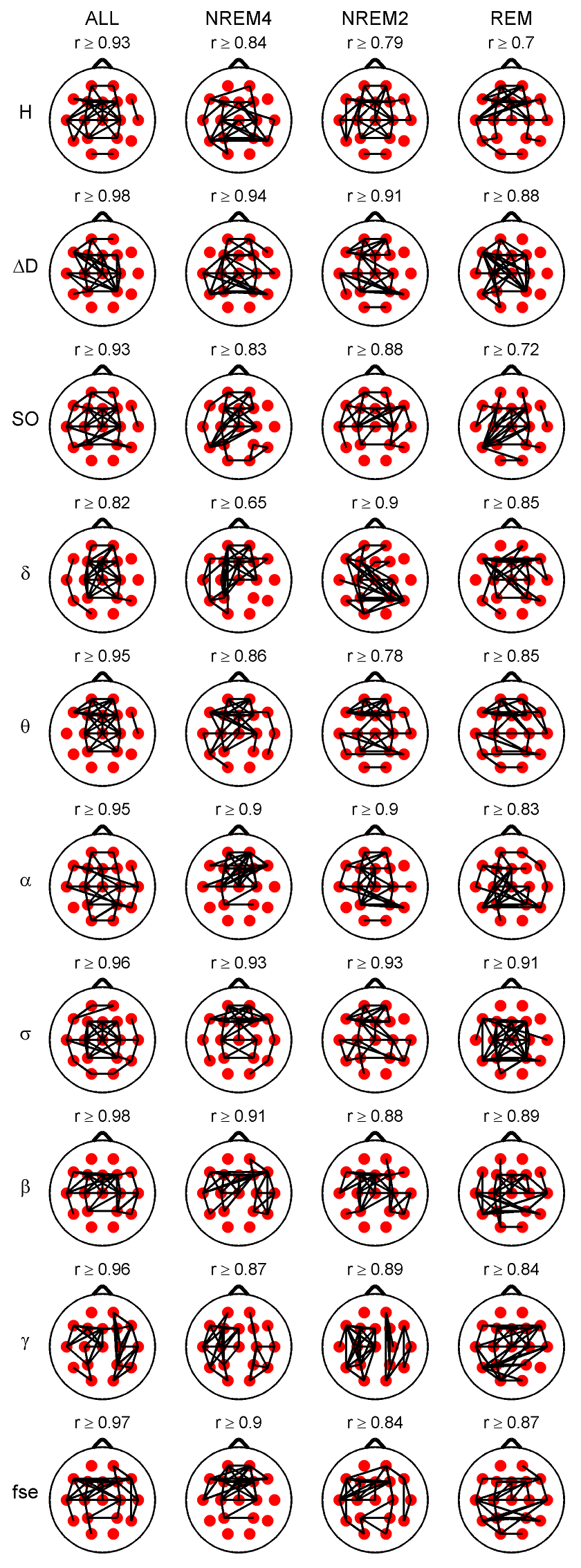
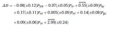
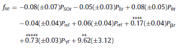
Fig. 2. Highest 35 inter-site correlations denoted by black lines drawn between the appropriate locations. Spearman’s correlation coefficients were calculated considering all sleep stages together (column ALL) as well as separately. Only significant (p < 0.05) correlations are depicted. Lowest presented correlation values can be found above the topographic maps. Relative band powers are denoted by the labels of the corresponding frequency bands.

3.2.2. Cross-correlation of measures

3.2.2.1. Cross-correlation between the fractal measures.
When all sleep stages were considered together strong negative crosscorrelations (p < 0.00001) between H and ΔD were found with weakest correlations in the occipital zone (Fig. 3). Evaluating sleep stages separately one could observe stronger and more significant correlation values for deeper sleep stages. During NREM4 lower values were found in the occipital and the fronto-polar regions. During NREM2 weakest correlations were found posteriorly. REM sleep showed non-significant negative correlations in the circumferential channels and non-significant but positive correlation in the F3, Fz, and F4 channels.

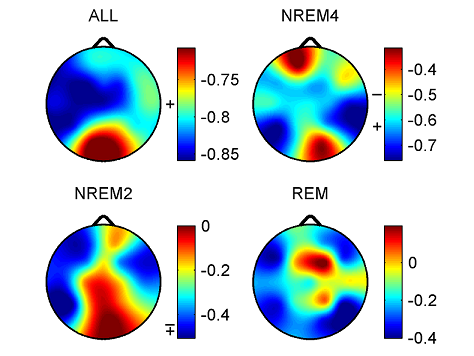
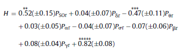
Fig. 3. Spearman cross-correlations between H and ΔD considering all sleep stages together as well as separately. Significant values (p < 0.05) are denoted on the left side of the color bars using the following notations: no sign (none of the values are significant); only + (all values are significant); + with a dash (only values below the dash are significant).

3.2.2.2. Cross-correlation between fractal and power spectral measures.
Results of cross-correlation analyses between fractal and power spectral measures are summarized in Fig. 4. Generally, a positive cross-correlation was observed between H and slower brain activities (SO and δ bands), while faster activities (above 4 Hz) were negatively correlated with the monofractal measureH. Higher and more significant correlations were found for deeper sleep stages. Overall, the strongest positive correlation was revealed for the relative power of the SO band, while the strongest negative correlation was found for the relative power of the theta band. Generally, weaker correlations appeared in the anterior channels during NREM4. During NREM2 stronger correlations (positive for the SO and negative for the θ band) were found in the anterior region while faster activities (σ, β, and  γ  bands) exhibited weakest correlations with H in posterior channels. During REM stronger positive correlation between slow activities (SO and δ bands) and H was found in the temporal and occipital channels while faster activities were negatively correlated with the monofractal measure H. Above the θ band stronger negative correlations were present in the circumferential channels decreasing around the vertex and even switching to positive correlation values in the case of α and γ bands.

Generally, correlations between ΔD and RBPs exhibited relationships with a sign opposite to that found for measure H. Namely, ΔD was negatively correlated with slow (SO and δ) while positively correlated with faster (above 4 Hz) activities. Similarly to H, more significant values appeared for deeper sleep stages. Compared to H, correlations of ΔD with slow activities were weaker and less significant. Highest positive correlation values between ΔD and P_Θr were found in the anterior channels regardless of sleep depth. Relative power of alpha and sigma bands exhibited strongest positive correlations with ΔD in the temporal channels. P_βr and P_γr showed strongest positive correlations with ΔD around the Fz channel during NREM4, while the nadirs of these correlations were found during REM sleep in the same region.
Inspection of cross-correlation maps between spectral edge frequency and the fractal measures indicated that these correlations reflect contribution of certain frequency bands in a compact way, such as in the case of the correlation between f_se and H during NREM4 where the minimum of correlations was found frontally.
To estimate the contribution of single frequency bands to the overall variation of compact measures, one must bear in mind that certain band powers are also correlated [11]. To control for this effect, we performed multiple linear regression (MLR) analyses with relative band powers as predictors and compact EEG measures as response variables. At this point we analyzed sleep stages together and only those channels where best classifications were predicted based on supplementary Table S1 and previous results presented in [95]. Thus, for H MLR was carried out in channel Cz with a result

and statistics F(7, 58) = 200.99, p < 0.00001, Std . Err . Est . = 0.01, R = 0.98, R² = 0.96, adjusted R2 = 0.96. For ΔD MLR was performed considering the T4 channel. The obtained result was 

with statistics F(7, 58) = 77.54, p < 0.00001, Std . Err . Est . = 0.12, R = 0.95, R² = 0.9, adjusted R² = 0.89. Finally, contribution of different frequency bands to the spectral edge frequency was tested in channel T6 with the result

and the following statistics F(7, 58) = 360, p < 0.00001, Std . Err . Est . = 1.23, R = 0.99, R² = 0.98, adjusted R² = 0.97. Coefficients of relative band powers were standardized and their standard errors were provided in brackets. Only coefficients with stars above them were significant with notation: ** (p < 0.01), *** (p < 0.001), **** (p < 0.0001) and ***** (p < 0.00001).

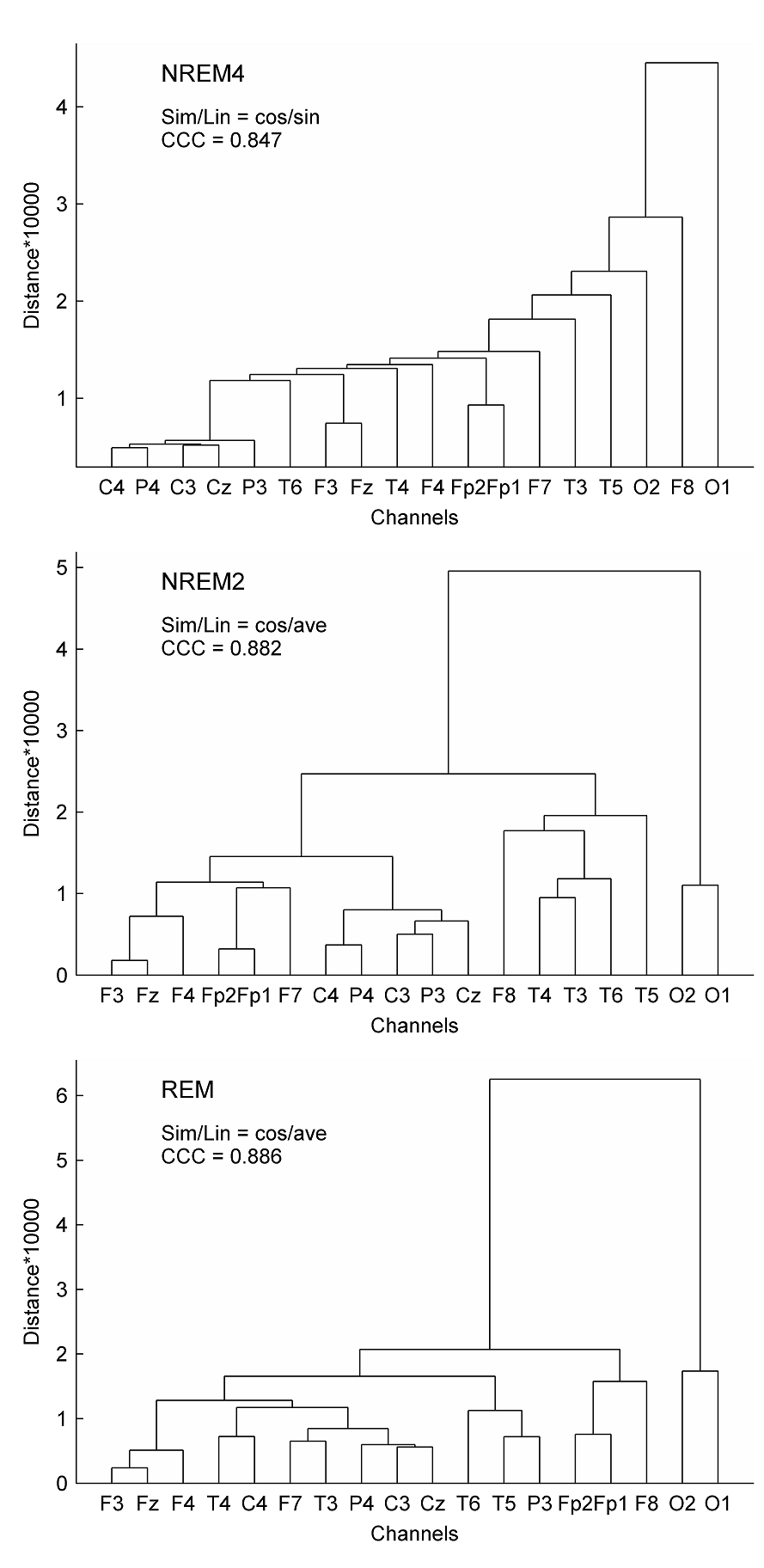
Fig. 4. Spearman cross-correlations between fractal and power spectral measures (PSMs). The left panel depicts results obtained for H. Cross-correlations between ΔD and PSMs are presented in the right panel. Sleep stages were considered together (columns denoted by ALL) as well as separately. Significant values (p < 0.05) are marked on the left side of the color bars using the following notations: no sign (none of the values are significant); only + (all values are significant); + with a dash (only values above/below the dash are significant). Relative band powers are denoted by the labels of the corr esponding frequency bands.

3.3. Clustering of channels and measures

Hierarchical channel cluster trees were generated for all three sleep stages and all EEG features separately using the best similarity and linkage combinations. Visual inspection of the dendrograms revealed both common and distinct channel clusters across sleep stages (see e.g. Fig. 5 for measure ΔD). For statistical evaluation channels were clustered into 4 and 9 clusters, respectively (supplementary Table S2).

Fig. 5. Dendrograms of EEG channels obtained using the multifractal measure ΔD. Hierarchical cluster trees were generated applying the best similarity/linkage (Sim/Lin) methods according to the cophenet correlation coefficient (CCC). For the abbreviation of Sim/Lin methods see Section 2.3.3.

As can be seen in Table S2 and Table 3, the 9-cluster analysis showed that most EEG features revealed proximity of symmetrical channels in the frontal region and during NREM4. As compared, during REM the symmetric channels were clustered together more posteriorly and circumferentially. Regardless of the sleep stage most of the measures (6–9 out of 10) indicated the proximity of F3–F4, C3–C4 and P3–P4 channels. The non-symmetrical Fz and Cz channels clustered together in much less cases. A more detailed examination of data in supplementary Table S2 unveiled that Fz tended to cluster with frontal F3 and F4 channels, while Cz mostly formed common clusters with the central channels C3 and C4. With regard to P_γr symmetric channels did not cluster together during NREM4 and NREM2 sleep stages but did so in REM sleep.

In the 4-cluster analysis, where all measures were considered separately, a rather uneven clustering of channels was found. Notably, in almost all cases there were channels (typically the circumferential ones such as: Fp1, Fp2, O1, O2, T5, T6) that formed individual clusters because of their large distance from the remaining EEG derivations. At the same time, several topographic features revealed by the above analyses could be verified. For example, highest P_σr values in parietal channels during NREM2 (Fig. 1) were reflected in a separate cluster formed by P3 and P4 channels. As another example disconnection of the hemispheres during NREM4 with regard to the relative power of the γ band (Fig. 2) was also supported by forming separate clusters over left and right hemispheres.

Hierarchical clustering of channels was also carried out using all measures together to minimize the effect of “outlier” channels and to assess topography of overall brain dynamics. Performing 4-cluster analysis of hierarchical channel cluster trees (Fig. 6) revealed symmetric channel clusters for all sleep stages (Table 4). In general, separate clusters were formed by anterior, central, temporal and posterior channels. Topographic boundaries of these clusters slightly varied across sleep stages.

When combining the fractal measures only (Table 5) or the relative band powers only (Table 6) less symmetrical and slightly different topographic grouping of channels was obtained, e.g. the separate cluster that was formed for the parietal channels during NREM2 using all measures together (Table 4) was not found using the fractal measures only.
In the next step we hierarchically clustered the computed EEG measures based on the 18 EEG channels (Fig. 6). In all sleep stages H was closest to relative band powers of slow activities (SO and δ bands). Measure ΔD was clustered with P_βr and P_γr during NREM4 and NREM2, while it formed a common cluster with P_αr and P_σr during REM. As expected from Eq. (14), with sleep deepening f_se was clustered with decreasing frequency bands, i.e. during REM f_se was clustered with P_γr, during NREM2 with P_αr and during NREM4 with P_θr.

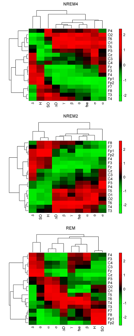
Fig. 6. Clustergrams generated for sleep stages NREM4, NREM2 and REM using group level medians of all measures in all channels. Heat maps and hereby the dendrograms were generated after z-standardization of the measures across the channels. Hierarchical channel cluster trees were generated using the cosine similarity metric and the unweighted average linkage method. The corresponding cophenet correlation coefficients (CCCs) were as follows: 0.749 (NREM4), 0.843 (NREM2) and 0.826 (REM). Measure dendrograms were constructed applying the Euclidean distance as a similarity measure and the unweighted average method for linkage (CCC: 0.959 (NREM4), 0974 (NREM2) and 0.886 (REM)). Relative band powers are denoted by the labels of the corresponding frequency bands.

3.4. Classification of sleep stages

Wecarried out a sleep stage classification using LDA both at individual and group levels. Maximal ˆK values across subjects (Fig. 7A) yielded best classifications for ΔD, f_se and P_βr features. There were 9 channels with highest ˆK values for ΔD and 8 channels for f_se. Kappa analysis did not reveal significant differences between the performances of these two measures at either channel (Table 7, imax test). Taking the average of ˆK values across subjects, ΔD provided the best performance in all channels (Fig. 7B). At the group level (Fig. 7C) highest ˆK values were also found for ΔD for most of the channels (except for T5, P3, P4, O1 and O2 channels) followed by measures f_se and P_βr. Comparing these three measures there were 8 channels (with a predominance of circumferential electrodes) where ΔD achieved significantly better performance compared to measures f_se and P_βr (Table 7, g test). Considering the individual level conditional ˆK values averaged across subjects ΔD showed best performance for NREM4 (Fig. 7D) as well as for NREM2 (Fig. 7E) in all channels while during REM ΔD, P_βr, P_γr and f_se revealed similar performance (Fig. 7F). Group level conditional ˆK values were presented in the last three columns of Fig. 7 (G, H, I). For NREM4 (Fig. 7G), ΔD showed the best classification results in all channels except for the occipital electrodes (Table 7, gcN4 test). During NREM2 best performance was also achieved for ΔD in most channels (13 channels) (Fig. 7H). Performance of ΔD significantly exceeded those of f_se and P_βr in 9 channels (Table 7, gcN2 test). By contrast, during REM f_se and P_βr significantly outperformed ΔD in all channels (Table 7, gcR test). Best classifications were obtained for measure P_βr in all channels. For all columns presented in Fig. 7 maximal ˆK values of ΔD were found in the circumferential channels (Table 8) with the best performance in T4 channel in 4 cases including mean ˆK values for the individual level (row B), ˆK values at the group level (row C) as well as conditional ˆK values in rows D and H. As can be seen in Table 8, best classification performance across EEG measures was found for ΔD considering all rows with the exception of rows (F, I) that is the conditional values for REM.

In (rows A–C) best classifications of ΔD exceeded 80% (peaking in 97.78% at individual level for subject #3) considering the overall accuracy measure.
Compared with other measures, H generally performed below the average with central peaks in ˆK values. In contrast to its general low level of performance it quite efficiently classified NREM4. When regarding results obtained for relative band powers (Fig. 7), higher overall performance was found for faster brain activities. In general, better classification results were found for NREM4 as compered with NREM2 and REM. Worst and non-significant (comparing against a random classifier) classification results were obtained at group level for sleep stage NREM2 using measures P_SOr (channel Fp2) and P_δr (channels F3, Fz, F4, F7, C4).

Fig. 7. Sleep stage classification results using linear discriminant analysis both at individual and group levels. (A) Maximal ˆK values taken across subjects. (B) Averaged individual ˆK values. (C) Group level ˆK values. (D) Individual conditional ˆK values averaged across subjects for sleep stage NREM4. (E) Individual conditional ˆK values averaged across subjects for sleep stage NREM2. (F) Individual conditional ˆK values averaged across subjects for REM sleep. (G) Group level conditional ˆK for NREM4 sleep. (H) Group level conditional ˆK for sleep stage NREM2. (I) Group level conditional ˆK for REM sleep. Relative band powers are denoted by the labels of the corresponding frequency bands.

4. Discussion

To our knowledge this is the first study providing a detailed comparison of fractal and power spectral features of the human EEG considering the effects of topography and sleep stages. Fractality of EEG signals was assessed using both monofractal and multifractal measures. Power spectral properties were described by relative band powers and in amore compact way by estimating the spectral edge frequency. Sleep was analyzed considering sleep stages NREM4, NREM2 and REM separately as well as together. Topography was assessed with regard to functional connectivity by analyzing interhemispheric differences and regional clustering of EEG derivations.

Our data indicate that despite of correlations between fractal and power spectral measures, fractal features carry additional information about EEG signals. Moreover, brain electrical activities are more complex than they could be fully described by a single monofractal exponent and therefore a multifractal approach may be more appropriate for modeling the fractal properties of brain dynamics.

A main and novel finding of the study is that the overall sleep stage discrimination capability of the multifractal measure is superior compared to the relative band powers, the compact power spectral measure f_se as well as the monofractal exponentH. Regarding overall accuracy ΔD exceeded 80% at the group level and achieved even 97.78% at the individual level. This finding speaks in favor of the individual level classification. Our results, in addition, indicate highest accuracy for the temporal channels which might surprise given that previous studies typically used central EEG channels for sleep stage classification.

4.1. Topographic and sleep stage-wise distribution of measures

Topographic distribution of the analyzed measures (Fig. 1) was in general agreement with expectations. Results obtained for the fractal measures were completely in agreement with those findings published in [95]. Higher H values occurred for deeper sleep stages, while ΔD showed an opposite trend indicating that brain electrical activities tend to be less multifractal and to posses longer memory properties during deeper sleep stages. The decrease of ΔD with the deepening of sleep was opposite to the behavior of another multifractal measure, the range of singularity strength in a previous study [63] where the multifractality of EEG signals was assessed analyzing the distribution of zero-crossings. This discrepancy indicates a need for a systematic comparison of different estimation methods for multifractal analysis of EEG signals. The H_NREM4 >H_NREM2 >H_REM trend was in agreement with results of previous studies that assessed the DFA λ exponent [53–55,86], the fractal exponent Κ [74] or the fractal dimension Df [73]. Namely, DFA exponent λ and κ increased with the deepening of sleep, while D_f exhibited the opposite trend. This suggests that the Hurst exponent estimated based on R/S statistics might be able to reflect the self-similarity properties of the sleep EEG, although the aforementioned trend could not be observed for H in [1]. Nevertheless, searching for the direct relationship between exact values of fractal measures and physiological processes has less sense, because of the already mentioned doubts related to estimation of fractal measures from time series of finite length. Even classification of actual brain dynamics into one of two types of fractional time series (fGn and fBm) is questionable. According to one part of the studies, fGn behavior of the sleep EEG could be conjectured based on DFA λ exponent values below 1 [54,55] or estimated Hurst exponents below 1 using the R/S statistics approach such as in the present study and in [1,95]. Other studies, on the contrary, indicated fBm nature of the human sleep EEG by revealing DFA κ exponent values above 1 [53,86] or fractal exponent values in the range 1 <κ <3[74]. These discrepancies might be due to different estimation settings and indicate a need for a comprehensive comparison of different approaches used for the assessment of fractal properties, including classification of EEG signals into one of two classes of fractional time series (fGn or fBm) as it was proposed in [24–26]. Moreover, we should keep in mind that sleep EEG signals exhibit multifractal properties and thus monofractal analysis can only give a measure of the largest of their fractal dimensions. The 1/f noise-like power spectrum ofEEGsignals can be distorted during different conditions by characteristic peak frequencies (e.g. due to the alpha rhythm or intensive sleep spindles) that could destroy the self-similar nature of EEG. Possible analyses for such cases were proposed in [29,57]. Finally, we should also note that recent investigations revealed effects of gender and age [68] as well as genetic contributions to long-range temporal correlations [60] in wake EEG signals. Therefore, effects of these factors should be investigated during different sleep stages as well. 
Our data on the topography of relative band powers only partially agreed with those published earlier. Slow activities characterizing NREM4 occurred in anterior channels, while faster activities during REM dominated posteriorly. This anteroposterior tendency is in general agreement with previous studies [21,22,45,96,97]. During NREM sleep stages, the fronto-central maximum of slow activities as well as the posterior maximum of theta activity and the parietal maximum of the sigma band are also in agreement with results presented in [31,92]. Nevertheless, the frontal maximum of alpha and beta band activities [31,92] was not supported by our results. Also, instead of the frontal sigma and beta peaks during REM in the study of Tinguely et al. [92] we found posterior and temporal peaks in these activities. We could neither confirm the frontal peak of NREM4 slow oscillation activity described by Happe et al. [40]. We assume that discrepancies might be due to methodological differences. Firstly, previous studies mostly used absolute power values while we used relative band powers. Secondly, several previous studies [31,45,92,96,97] evaluated NREM sleep stages together, while we examined NREM4 and NREM2 stages separately. Nevertheless, we were able to confirm the known topographic spectral features of characteristic sleep EEG patterns. The revealed fronto-central peak in delta activity during NREM4 and NREM2 likely reflects delta waves and K-complexes [39,40]. The parietal peak of sigma activity during NREM2 may stand for fast sleep spindles [20,98,100]. At the same time no salient topographic feature could be related to frontal slow spindle activity. Vertex peaks in delta and theta bands during REM sleep likely reflects saw tooth waves, characteristic EEG patterns during REM with a know central maximum [99].

4.2. Cross-correlations between measures

In our previous study [95] we found a tendency for an overall negative cross-correlation between H and ΔD. In that study we also revealed a specific topography of this relationship. Here we extend the characterization of the cross-correlation between H and ΔD by assessing sleep stages separately. Combining all sleep stages we found a strong negative correlation between H and ΔD with a nadir in the posterior channels (Fig. 3). As revealed by the sleep stage-wise analysis NREM2 and NREM4 contributed most to this occipital nadir. As compared to NREM4 weaker and less significant correlations emerged during NREM2. During REM there was a further weakening of correlations with a non-significant positive peak in the F3, Fz, F4 channels.
To reveal how spectral properties are reflected in fractal measures, we performed cross-correlation analysis between these measures (Fig. 4). Measure H exhibited positive correlation with relative powers of slow activities (especially P_SOr), while it mostly showed negative correlation with faster activities. More significant values tended to occur for slower activities (except P_δr) and for deeper sleep stages. All these findings support the theory that H is linearly related to the spectral exponent κ (see Section 2.2.2.1). Parameter κ can be estimated by plotting the power spectrum on the log-log scale and by fitting a straight line to this plot. The slope of this line is equal to -κ. This indicates that higher amount of slow activities and lower amount of faster activities result in higher κ and H values and vice versa. The log–log plot of the power spectrum produces several points at higher frequencies and only few points at lower frequencies. Hence, the fitting of a straight line is much more affected by lower frequencies which might be the cause of more significant correlations of H with slower brain activities. Thus the correlation withHdepends not only on the position, width and power amount of a given frequency band but it is also affected by properties of other bands. This provides an explanation why P_δr exhibited weaker and less significant correlations with H as it could have been expected. As it could be conjectured from the overall negative cross-correlation between the fractal measures, ΔD generally revealed opposite correlations with power spectral measures compared to those of H. That is,ΔD was negatively correlated with slow activities and positively correlated with RBPs of higher frequency bands. Additionally, faster activities (> 4 Hz) showed more significant correlations with ΔD as compared to slower activities and for deeper sleep stages. All this suggests that slower EEG patterns tend to make the amplitude distribution more even, while the opposite is true for faster EEG patterns. Characteristic topography of cross-correlations between H and ΔD were also reflected in crosscorrelations between the fractal measures and RBPs, e.g. one of the most striking topographic features of cross-correlations between fractal measures and relative band powers could be observed for REM sleep in the fronto-central region where weakest correlations occurred. This might explain weak and non-significant positive cross-correlation between the two fractal measures during REM. Multiple linear regressions supported results of cross-correlation analysis between fractal and RBP measures by revealing contribution of individual RBPs to the compact EEG measures. We found a positive contribution of slow (SO and Δ bands) activities to H. Out of the faster activities P_αr and P_γr contributed positively while P_θr, P_σr and P_βr contributed negatively to the same measure. The positive contribution of P_αr and P_γr might be explained by the observed weak positive cross-correlation between these measures and H during REM sleep in the central zone (see Fig. 4). Highest coefficients were revealed for P_SOr and P_θr. Considering ΔD, negative and non-significant contribution of slow activities was obtained. Positive coefficients were found for faster activities (above 4 Hz) reaching the significance level only for P_θr. In addition, expected results were also found considering f_se as a predicted variable. Highest positive and significant coefficients were found for two fastest activities (P_βr and P_γr). Fraction of variation that could be explained by the relative band powers was highest in case of f_se (adjusted R² = 0.97), while the worst regression result was found for ΔD (adjusted R² = 0.89). This finding could have been anticipated since f_se is directly computed from power spectra and H may be related to the power spectrum, while ΔD reflects the amplitude distribution of time series. Distance of compact EEG features and RBPs was also analyzed by hierarchical clustering of the measures using group level medians in all channels (Fig. 6). These results were in agreement with those obtained by cross-correlation analyses and MLR. Namely, H was clustered with relative powers of slow brain activities (SO and δ frequency bands) in all sleep stages, while ΔD tended to cluster with faster activities (β and γ bands during NREM4 and NREM2; and bands during REM sleep). 
A direct comparison of our correlation results (between H and spectral measures) with those of previous investigators is not possible since previous investigators used different measures and only few EEG channels. Nevertheless, our results regarding the correlation between H and power spectral measures could be related to those results by Pereda et al. [73] who revealed a similar trend of measures D₂ and D_f across sleep stages and a negative crosscorrelation between D₂ and powers of slower frequency bands [74]. Another study revealing negative cross-correlation between D₂ and DFA exponent λ and negative cross-correlation between D₂ and slower activities [86] also seem to be in accordance with our data. On the contrary, the weak positive cross-correlation between D₂ and Κ during NREM4 and NREM3 found in [74] would suggest negative correlation between H and slow activities. As far as we know there are no studies in the literature examining the relationship between multifractality and spectral measures of sleep EEG.

4.3. Interhemispheric differences and inter-site correlations

In the present study we also compared inter-site correlations (Fig. 2) and interhemispheric differences of fractal and power spectral measures (Table 2). Surprisingly interhemispheric differences of specific measures varied with sleep stages and locations more than expected. In addition, it is difficult to relate these results to previous data where sleep stages were combined and/or EEG recordingwaslimited to a few channels. Nevertheless,wewere able to reveal some coherent tendencies regarding the interhemispheric differences of spectral powers, e.g.weobserved a right-hemisphere predominance of SO duringNREM4which might be related to those results by Sekimoto et al. [84] finding predominance of 0.5–2 Hz activity over the right hemisphere during all night sleep. At the same time delta activity on the left side tended to predominate in each sleep stage. During NREM4 and NREM2 we found higher theta activity on the right side, while during REM theta predominated on the left side corroborating the findings of Roth et al. [82]. The majority of interhemispheric comparisons of H and ΔD were not significant. Previous investigators revealed interhemispheric asymmetries for measures D₂, L₁ and D_f considering C3–C4 channels [73] and interhemishperic differences for D2 in C3–C4, T3–T4 and O1–O2 locations [50]. Differences between earlier and the present data might be due to several methodological differences. Inter-site correlations of RBPs (Fig. 2) partially agreed with those results of coherence analyses revealed in [2,30,46]. Specifically, we found stronger interhemispheric P_γr correlations during REM compared to NREM4 and NREM2, a finding similar to obtained by Achermann and Borbély [2]. However, this result should be regarded with caution since disconnection of the hemispheres during NREM4 and NREM2 sleep regarding P_γr might also occur due to the application of two separate references [27,36,43].
As expected, less significant differences were found for the symmetrical channel pairs as compared with the non-symmetrical channel pair Fz–Cz. These results indicate stronger functional connectivity between the homologous hemispheric regions that could be mediated to a large part by the corpus callosum and other commissural pathways [93,94]. During NREM4 most significant interhemispheric differences were found for occipital and parietal symmetrical channel pairs (Table 2). Results in the interhemisperic analysis were confirmed by the inter-site correlation analysis (Fig. 2) revealing strongest correlations between the anterior channels during NREM4. During NREM2 and REM strongest correlations were located more posteriorly. The 9-cluster analysis (Table S2, Table 3) also confirmed this trend by revealing a tendency of clustering together the frontal symmetrical channels during NREM4 and the posterior homologous channels during REM sleep. These findings suggest stronger interhemispheric functional connectivity anteriorly during NREM4 and posteriorly during REM sleep. Topography of inter-site correlations of compact EEG features (including fractal measures and f_se) reflect those of RBPs to some extent but due to the compression of information several properties are lost, e.g. the disconnection of the hemispheres during NREM4 and NREM2 regarding the gamma band activity cannot be revealed from compact features. The 4-cluster analysis revealed similar channel clusters (anterior, posterior, central and temporal) for the combined fractal measures (Table 5) and for the combined RBPs (Table 6). Nevertheless, there were some differences between these two latter clusterings which could be related to the aforementione d information loss. For example, the separate cluster that was formed for the parietal channels using the RBP measures was modified by clustering the parietal channels together with central derivations based on combination of fractal measures. Combination of fractal features and PSMs (Fig. 6 and Table 4) provided more symmetrical topographic clusters than those obtained for the combined fractal measures or the combined RBP measures (as well as combined PSMs: data not presented) alone. Nevertheless, all these results indicate a re-organization of functional connectivity between brain regions across sleep stages.

4.4. Discriminability of sleep stages

Sleep stage discrimination capabilities of EEG features were tested in each channel both at individual and group levels (see Fig. 7 and Tables 7 and 8). Results indicate best overall classifications for ΔD followed by f_se and P_βr. This could have been assumed from Table S1 since these three measures tended to reveal most significant differences for all sleep stage pairs. Superior performance of ΔD and f_se is in agreement with results obtained previously for the entropy of amplitudes and spectral edge frequency measures [28]. In the present study best classifications for ΔD were revealed for the temporal channels. Measure H performed below the average considering all measures. This result is in contrast with a previous study [91] finding a superior performance of two other monofractal measures (the fractal exponent and the fractal dimension) when compared to spectral measures. To our surprise, worst classification performance was obtained for the relative band power of slow activities. This might be explained by confining the δ band to the 1- 4Hz range and considering slow oscillations (0.5–1 Hz) separately. The outstanding performance of ΔD, f_se and P_βr indicate that it is the faster rather than the slow activities that might be of superior performance in the classification of sleep stages. As expected, better classifications were achieved at the individual level as compared to the group level, a finding that could be related to the considerable individual variability of sleep EEG features [23,32].
Examination of conditional ˆK^ values revealed that high overall performance of ΔD was achieved due to significantly better classification of the NREM4 sleep stage. Comparatively, measure ΔD was found to be less efficient in classifying NREM2 and REM. Nevertheless, these latter stages could be classified better based on specific EEG measures at specific locations, e.g. best classification of NREM2 was revealed using P_σr centrally (Fig. 7H) and best classification of REM was found using P_βr in frontal channels (Fig. 7I). Thus we assume that overall sleep stage classification performance could be improved by combining different measures at different locations. In addition application of more sophisticated classification paradigms and their combinations could be also beneficial. Polygraphic information (EMG, EOG, ECG) might obviously improve the sleep stage classification performance. Nevertheless, developing sleep stage classifications not relying on polygraphic information might be useful for invasive intracranial EEG recordings where polygraphy is typically not available.
In this study we assessed the relatively well-distinguishable sleep stages NREM4, NREM2 and REM. It remains to be tested whether other sleep stages (NREM1 and NREM3), waking states or the wake-sleep transition can be classified and detected with a same performance using fractal measures alone or combined with other features.

Conflict of interest

The authors declare that they have no competing financial interests.

Acknowledgment
This research was supported by the Faculty of Information Technology and the Jedlik Laboratories of the Pázmány Péter Catholic University, Budapest, Hungary.

Appendix A. Supplementary data
Supplementary data associated with this article can be found, in the online version, at doi:10.1016/j.brainresbull.2010.12.005.

References

[1] R. Acharya, O. Faust, N. Kannathal, T. Chua, S. Laxminarayan, Non-linear analysis of EEG signals at various sleep stages, Comput. Methods Progr. Biomed. 80 (1) (2005) 37–45.

[2] P. Achermann, A. Borbély, Coherence analysis of the human sleep electroencephalogram, Neuroscience 85 (4) (1998) 1195–1208.

[3] P. Achermann, A. Borbély, Low-frequency (<1 Hz) oscillations in the human sleep electroencephalogram, Neuroscience 81 (1) (1997) 213–222.

[4] P. Bak, How Nature Works: The Science of Self-organized Criticality, Oxford University Press, Oxford, 1997.

[5] P. Bak, C. Tang, K. Wiesenfeld, Self-organized criticality: an explanation of the 1/f noise, Phys. Rev. Lett. 59 (4) (1987) 381–384.

[6] P. Bak, C. Tang, K. Wiesenfeld, Self-organized criticality, Phys Rev A 38 (1) (1988) 364–374.

[7] A.L. Barabási, H.E. Stanley, Fractal Concepts in Surface Growth, Cambridge University Press, Cambridge, 1994.

[8] J.B. Bassingthwaighte, L.S. Liebovitch, B.J. West, Fractal Physiology, Oxford University Press, New York, 1994.

[9] C. Bédard, H. Kröger, A. Destexhe, Does the 1/f frequency scaling of brain signals reflect self-organized critical states? Phys. Rev. Lett. 97 (11) (2006) 118102.

[10] J. Beggs, D. Plenz, Neuronal avalanches in neocortical circuits, J. Neurosci. 23 (35) (2003) 11167–11177.

[11] O. Benoit, A. Daurat, J. Prado, Slow (0.7–2 Hz) and fast (2–4 Hz) delta components are differently correlated to theta, alpha and beta frequency bands during NREM sleep, Clin. Neurophysiol. 111 (12) (2000) 2103–2106.

[12] J. Beran, Statistics for Long-Memory Processes, 1st ed., Chapman & Hall/CRC, New York, 1994.

[13] T. Boji´ c, A. Vuckovic, A. Kalauzi, Modeling EEG fractal dimension changes in wake and drowsy states in humans—a preliminary study, J. Theor. Biol. 262 (2) (2010) 214–222.

[14] R. Cerf, A. Daoudi, M. Ould Hénoune, E. el Ouasdad, Episodes of low-dimensional self-organized dynamics from electroencephalographic alpha-signals, Biol. Cybern. 77 (4) (1997) 235–245.

[15] Z. Chen, K. Hu, P. Carpena, P. Bernaola-Galvan, H. Stanley, P. Ivanov, Effect of nonlinear filters on detrended fluctuation analysis, Phys. Rev. E Stat. Nonlin. Soft Matter Phys. 71 (1 Pt 1) (2005) 011104.

[16] Z. Chen, P. Ivanov, K. Hu, H. Stanley, Effect of nonstationarities on detrended fluctuation analysis, Phys. Rev. E Stat. Nonlin. Soft Matter Phys. 65 (4 Pt 1) (2002) 041107.

[17] D. Chialvo, P. Bak, Learning from mistakes, Neuroscience 90 (4) (1999) 1137–1148.

[18] R.G. Congalton, K. Green, Assessing the Accuracy of Remotely Sensed Data: Principles and Practices, 2nd ed., CRC Press, Boca Raton, 2008.

[19] P. Couto, Assessing the accuracy of spatial simulation models, Ecol. Modell. 167 (1–2) (2003) 181–198.

[20] L. De Gennaro, M. Ferrara, Sleep spindles: an overview, Sleep Med. Rev. 7 (5) (2003) 423–440.

[21] L. De Gennaro, M. Ferrara, G. Curcio, R. Cristiani, M. Bertini, Cortical EEG topography of REM onset: the posterior dominance of middle and high frequencies, Clin. Neurophysiol. 113 (4) (2002) 561–570.

[22] L. De Gennaro, M. Ferrara, G. Curcio, R. Cristiani, Antero-posterior EEG changes during the wakefulness-sleep transition, Clin. Neurophysiol. 112 (10) (2001) 1901–1911.

[23] L. De Gennaro, M. Ferrara, F. Vecchio, G. Curcio, M. Bertini, An electroencephalographic fingerprint of human sleep, Neuroimage 26 (1) (2005) 114–122.

[24] D. Delignieres, S. Ramdani, L. Lemoine, K. Torre, M. Fortes, G. Ninot, Fractal analyses for ‘short’ time series: a re-assessment of classical methods, J. Math. Psychol. 50 (6) (2006) 525–544.

[25] A. Eke, P. Herman, L. Kocsis, L. Kozak, Fractal characterization of complexity in temporal physiological signals, Physiol. Meas. 23 (1) (2002) R1–38.

[26] A. Eke, P. Hermán, J. Bassingthwaighte, G. Raymond, D. Percival, M. Cannon, I. Balla, C. Ikrényi, Physiological time series: distinguishing fractal noises from motions, Pflugers Arch. 439 (4) (2000) 403–415.

[27] M. Essl, P. Rappelsberger, EEG coherence and reference signals: experimental results and mathematical explanations, Med. Biol. Eng. Comput. 36 (4) (1998) 399–406.

[28] J. Fell, J. Röschke, K. Mann, C. Schäffner, Discrimination of sleep stages: a comparison between spectral and nonlinear EEG measures, Electroencephalogr. Clin. Neurophysiol. 98 (5) (1996) 401–410.

[29] T.C. Ferree, R.C. Hwa, Power-law scaling in human EEG: relation to Fourier power spectrum, Neurocomputing 52–54 (2003) 755–761.

[30] R. Ferri, F. Rundo, O. Bruni, M. Terzano, C. Stam, Regional scalp EEG slowwave synchronization during sleep cyclic alternating pattern A1 subtypes, Neurosci. Lett. 404 (3) (2006) 352–357.

[31] L. Finelli, A. Borbély, P. Achermann, Functional topography of the human nonREM sleep electroencephalogram, Eur. J. Neurosci. 13 (12) (2001) 2282–2290.

[32] L. Finelli, P. Achermann, A. Borbély, Individual, ‘fingerprints’ in human sleep EEG topography, Neuropsychopharmacology 25 (5 Suppl.) (2001) S57–S62.

[33] W. Freeman, L. Rogers, M. Holmes, D. Silbergeld, Spatial spectral analysis of human electrocorticograms including the alpha and gamma bands, J. Neurosci. Methods 95 (2) (2000) 111–121.

[34] W. Freeman, M. Holmes, B. Burke, S. Vanhatalo, Spatial spectra of scalp EEG O. Jenni, E. van Reen, M. Carskadon, Regional differences of the sleep electroencephalogram and EMG from awake humans, Clin. Neurophysiol. 114 (6) (2003) 1053–1068.

[35] J. González, A. Gamundi, R. Rial, M. Nicolau, L. de Vera, E. Pereda, Nonlinear, fractal, and spectral analysis of the EEG of lizard, Gallotia galloti, Am. J. Physiol. 277 (1 Pt 2) (1999) R86–R93.

[36] S. Gudmundsson, T. Runarsson, S. Sigurdsson, G. Eiriksdottir, K. Johnsen, Reliability of quantitative EEG features, Clin. Neurophysiol. 118 (10) (2007) 2162–2171.

[37] G. Gurman, Assessment of depth of general anesthesia. Observations on processed EEG and spectral edge frequency, Int. J. Clin. Monit. Comput. 11 (3) (1994) 185–189.

[38] G. Gurman, S. Fajer, A. Porat, M. Schily, A. Pearlman, Use of EEG spectral edge as index of equipotency in a comparison of propofol and isoflurane for maintenance of general anaesthesia, Eur. J. Anaesthesiol. 11 (6) (1994) 443–448.

[39] P. Halasz, K-complex, a reactive EEG graphoelement of NREM sleep: an old chap in a new garment, Sleep Med. Rev. 9 (5) (2005) 391–412.

[40] S. Happe, P. Anderer, G. Gruber, G. Klösch, B. Saletu, J. Zeitlhofer, Scalp topography of the spontaneous K-complex and of delta-waves in human sleep, Brain Topogr. 15 (1) (2002) 43–49.

[41] T. Higuchi, Relationship between the fractal dimension and the power law index for a time series: a numerical investigation, Physica D: Nonlin. Phenomena 46 (2) (1990) 254–264.

[42] K. Hu, P. Ivanov, Z. Chen, P. Carpena, H. Stanley, Effect of trends on detrended fluctuation analysis, Phys. Rev. E: Stat. Nonlin. Soft Matter Phys. 64 (1 Pt 1) (2001) 011114.

[43] S. Hu, M. Stead, Q. Dai, G. Worrell, On the recording reference contribution to EEG correlation, phase synchorony, and coherence, IEEE Trans. Syst. Man. Cybern. B Cybern. (2010).

[44] H.E. Hurst, Long term storage capacity of reservoirs, Trans. Am. Soc. Civil Eng. 116 (1951) 770–799.

[45] O. Jenni, E. van Reen, M. Carskadon, Regional differences of the sleep electroencephalogram in adolescents, J. Sleep Res. 14 (2) (2005) 141–147.

[46] M. Kamin´ ski, K. Blinowska, W. Szclenberger, Topographic analysis of coherence and propagation of EEG activity during sleep and wakefulness, Electroencephalogr. Clin. Neurophysiol. 102 (3) (1997) 216–227.

[47] H. Kantz, T. Schreiber, Nonlinear Time Series Analysis, 2nd ed., Cambridge University Press, Cambridge, New York and Melbourne, 2003.

[48] S. Katsev, I. L’Heureux, Are Hurst exponents estimated from short or irregular time series meaningful? Comput. Geosci. (2003) 1085–1089.

[49] V.G. Kiselev, K.R. Hahn, D.P. Auer, Is the brain cortex a fractal? Neuroimage 20 (3) (2003) 1765–1774.

[50] T. Kobayashi, S. Madokoro, K. Misaki, J. Murayama, H. Nakagawa, Y. Wada, Interhemispheric differences of the correlation dimension in a human sleep electroencephalogram, Psychiatry Clin. Neurosci. 56 (3) (2002) 265–266.

[51] V. Kulish, A. Sourin, O. Sourina, Human electroencephalograms seen as fractal time series: mathematical analysis and visualization, Comput. Biol. Med. 36 (3) (2006) 291–302.

[52] J. Landis, G. Koch, The measurement of observer agreement for categorical data, Biometrics 33 (1) (1977) 159–174.

[53] J.M. Lee, D.J. Kim, I.Y. Kim, K.S. Park, S.I. Kim, Nonlinear-analysis of human sleep EEG using detrended fluctuation analysis, Med. Eng. Phys. 26 (9) (2004) 773–776.

[54] S. Leistedt, M. Dumont, N. Coumans, J. Lanquart, F. Jurysta, P. Linkowski, The modifications of the long-range temporal correlations of the sleep EEG due to major depressive episode disappear with the status of remission, Neuroscience 148 (3) (2007) 782–793.

[55] S. Leistedt, M. Dumont, J.P. Lanquart, F. Jurysta, P. Linkowski, Characterization of the sleep EEG in acutely depressed men using detrended fluctuation analysis, Clin. Neurophysiol. 118 (4) (2007) 940–950.

[56] C.D. Lewis, G.L. Gebber, P.D. Larsen, S.M. Barman, Long-term correlations in the spike trains of medullary sympathetic neurons, J. Neurophysiol. 85 (4) (2001) 1614–1622.

[57] D. Lin, A. Sharif, H. Kwan, Scaling and organization of electroencephalographic background activity and alpha rhythm in healthy young adults, Biol. Cybern. 95 (5) (2006) 401–411.

[58] K. Linkenkaer-Hansen, V. Nikouline, J. Palva, R. Ilmoniemi, Long-range temporal correlations and scaling behavior in human brain oscillations, J. Neurosci. 21 (4) (2001) 1370–1377.

[59] K. Linkenkaer-Hansen, V. Nikulin, J. Palva, K. Kaila, R. Ilmoniemi, Stimulusinduced change in long-range temporal correlations and scaling behaviour of sensorimotor oscillations, Eur. J. Neurosci. 19 (1) (2004) 203–211.

[60] K. Linkenkaer-Hansen, D. Smit, A. Barkil, T. van Beijsterveldt, A. Brussaard, D. Boomsma, A. van Ooyen, E. de Geus, Genetic contributions to long-range temporal correlations in ongoing oscillations, J. Neurosci. 27 (50) (2007) 13882–13889.

[61] C. Long, N. Shah, C. Loughlin, J. Spydell, R. Bedford, A comparison of EEG determinants of near-awakening from isoflurane and fentanyl anesthesia. Spectral edge, median power frequency, and delta ratio, Anesth. Analg. 69 (2) (1989) 169–173.

[62] S.B. Lowen, L.S. Liebovitch, J.A. White, Fractal ion-channel behavior generates fractal firing patterns in neuronal models, Phys. Rev. E Stat. Phys. Plasmas Fluids Relat. Interdiscip. Top. 59 (5 Pt B) (1999) 5970–5980.

[63] Q.L. Ma, X.B. Ning, J. Wang, C.H. Bian, A new measure to characterize multifractality of sleep electroencephalogram, Chin. Sci. Bull. 51 (24) (2006) 3059–3064.

[64] B.B. Mandelbrot, M.S. Taqqu, Robust R/S analysis of long-run serial correlation, in: Proceedings of the 42nd Session of the International Statistical Institute, 48, Book 2, Manila, 1979, pp. 69–104.

[65] B.B. Mandelbrot, The Fractal Geometry of Nature, 1st ed., W.H. Freeman and Company, New York, 1982.

[66] M. Massimini, R. Huber, F. Ferrarelli, S. Hill, G. Tononi, The sleep slow oscillation as a traveling wave, J. Neurosci. 24 (31) (2004) 6862–6870.

[67] V. Nikulin, T. Brismar, Long-range temporal correlations in alpha and beta osc illations: effect of arousal level and test-retest reliability, Clin. Neurophysiol. 115 (8) (2004) 1896–1908.

[68] V. Nikulin, T. Brismar, Long-range temporal correlations in electroencephalographic oscillations: Relation to topography, frequency band, age and gender, Neuroscience 130 (2) (2005) 549–558.

[69] M. Palus, Nonlinearity in normal human EEG: cycles, temporal asymmetry, nonstationarity and randomness, not chaos, Biol. Cybern. 75 (5) (1996) 389–396.

[70] A. Pellionisz, Neural geometry: towards a fractal model of neurons, in: R.M.J. Cotterill (Ed.), Models of Brain Function, Cambridge University Press, Cambridge, New York and Melbourne, 1989, pp. 453–464.

[71] C. Peng, S. Havlin, H. Stanley, A. Goldberger, Quantification of scaling exponents and crossover phenomena in nonstationary heartbeat time series, Chaos 5 (1) (1995) 82–87.

[72] C.K. Peng, S.V. Buldyrev, S. Havlin, M. Simons, H.E. Stanley, A.L. Goldberger, Mosaic organization of DNA nucleotides, Phys. Rev. E 49 (2) (1994) 1685.

[73] E. Pereda, A. Gamundi, M. Nicolau, R. Rial, J. González, Interhemispheric differences in awake and sleep human EEG: a comparison between non-linear and spectral measures, Neurosci. Lett. 263 (1) (1999) 37–40.

[74] E. Pereda, A. Gamundi, R. Rial, J. González, Non-linear behaviour of human EEG: fractal exponent versus correlation dimension in awake and sleep stages, Neurosci. Lett. 250 (2) (1998) 91–94.

[75] L. Poupard, R. Sartčne, J. Wallet, Scaling behavior in beta-wave amplitude modulation and its relationship to alertness, Biol. Cybern. 85 (1) (2001) 19–26.

[76] G. Rangarajan, M. Ding, Integrated approach to the assessment of long range correlation in time series data, Phys. Rev. E Stat. Phys. Plasmas Fluids Relat. Interdiscip. Top. 61 (5A) (2000) 4991–5001.

[77] P. Rapp, A. Albano, T. Schmah, L. Farwell, Filtered noise can mimic lowdimensional chaotic attractors, Phys. Rev. E Stat. Phys. Plasmas Fluids Relat. Interdiscip. Top. 47 (4) (1993) 2289–2297.

[78] A. Rechtschaffen, A. Kales, Amanual of standardized terminology, techniques and scoring system for sleep stages of human subjects, Bethesda, MD, U.S. National Institute of Neurological Diseases and Blindness, Neurol. Inform. Netw. (1968).

[79] A. Rényi, Probability Theory, North Holland, Amsterdam, 1971.

[80] P.A. Robinson, C.J. Rennie, J.J. Wright, H. Bahramali, E. Gordon, D.L. Rowe, Prediction of electroencephalographic spectra from neurophysiology, Phys. Rev. E 63 (2) (2001) 021903.

[81] P.A. Robinson, C.J. Rennie, D.L. Rowe, Dynamics of large-scale brain activity in normal arousal states and epileptic seizures, Phys. Rev. E 65 (4) (2002) 041924.

[82] C. Roth, P. Achermann, A. Borbély, Frequency and state specific hemispheric asymmetries in the human sleep EEG, Neurosci. Lett. 271 (3) (1999) 139–142.

[83] T. Schreiber, A. Schmitz, Surrogate time series, Physica D: Nonlin. Phenom. 142 (3–4) (2000) 346–382.

[84] M. Sekimoto, M. Kato, N. Kajimura, T. Watanabe, K. Takahashi, T. Okuma, Asymmetric interhemispheric delta waves during all-night sleep in humans, Clin. Neurophysiol. 111 (5) (2000) 924–928.

[85] M. Shadlen, W. Newsome, The variable discharge of cortical neurons: implications for connectivity, computation, and information coding, J. Neurosci. 18 (10) (1998) 3870–3896.

[86] Y. Shen, E. Olbrich, P. Achermann, P.F. Meier, Dimensional complexity and spectral properties of the human sleep EEG, Clin. Neurophysiol. 114 (2) (2003) 199–209.

[87] Y. Shu, A. Hasenstaub, D. McCormick, Turning on and off recurrent balanced cortical activity, Nature 423 (6937) (2003) 288–293.

[88] S. Spasic, A. Kalauzi, G. Grbic, L. Martac, M. Culic, Fractal analysis of rat brain activity after injury, Med. Biol. Eng. Comput. 43 (3) (2005) 345–348.

[89] C. Stam, J. Pijn, P. Suffczynski, F. Lopes da Silva, Dynamics of the human alpha rhythm: evidence for non-linearity? Clin. Neurophysiol. 110 (10) (1999) 1801–1813.

[90] C. Stam, Nonlinear dynamical analysis of EEG and MEG: review of an emerging field, Clin. Neurophysiol. 116 (10) (2005) 2266–2301.

[91] K. Susmáková, A. Krakovská, Discrimination ability of individual measures used in sleep stages classification, Artif. Intell. Med. 44 (3) (2008) 261–277.

[92] G. Tinguely, L.A. Finelli, H.P. Landolt, A.A. Borbely, P. Achermann, Functional EEGtopography in sleep and waking: state-dependent and state-independent features, Neuroimage 32 (1) (2006) 283–292.

[93] V. Vyazovskiy, P. Achermann, A. Borbély, I. Tobler, Interhemispheric coherence of the sleep electroencephalogram in mice with congenital callosal dysgenesis, Neuroscience 124 (2) (2004) 481–488.

[94] V. Vyazovskiy, I. Tobler, Regional differences in NREM sleep slow-wave activity in mice with congenital callosal dysgenesis, J. Sleep Res. 14 (3) (2005) 299–304.

[95] B. Weiss, Z. Clemens, R. Bódizs, Z. Vágó, P. Halász, Spatio-temporal analysis of monofractal and multifractal properties of the human sleep EEG, J. Neurosci. Methods 185 (1) (2009) 116–124.

[96] E. Werth, P. Achermann, A. Borbély, Brain topography of thehumansleep EEG: antero-posterior shifts of spectral power, Neuroreport 8 (1) (1996) 123–127.

[97] E. Werth, P. Achermann, A. Borbély, Fronto-occipital EEG power gradients in human sleep, J. Sleep Res. 6 (2) (1997) 102–112.

[98] E. Werth, P. Achermann, D. Dijk, A. Borbély, Spindle frequency activity in the sleep EEG: individual differences and topographic distribution, Electroencephalogr. Clin. Neurophysiol. 103 (5) (1997) 535–542.

[99] A. Yasoshima, H. Hayashi, S. Iijima, Y. Sugita, Y. Teshima, T. Shimizu, Y. Hishikawa, Potential distribution of vertex sharp wave and saw-toothed wave on the scalp, Electroencephalogr. Clin. Neurophysiol. 58 (1) (1984) 73–76.

[100] J. Zeitlhofer, G. Gruber, P. Anderer, S. Asenbaum, P. Schimicek, B. Saletu, Topographic distribution of sleep spindles in young healthy subjects, J. Sleep Res.6 (3) (1997) 149–155.